Musical Consonance from Frequency Interactions
Better resources exist - see references below. Content generated via LLM collaboration - see authorship note.
How Musical Consonance Emerges from Frequency Interactions
This figure explains musical consonance and dissonance by linking auditory physiology, harmonic spectra, and frequency-domain interaction structure. It is organized as a causal sequence: ear response → musical outcome → physical mechanism. Each panel answers a different question, and the relationships between panels are integrative, not coordinate-aligned.
All calculations use a reference fundamental frequency of f₀ = 200 Hz (approximately G3) with 30 harmonic partials, and employ a simplified Plomp–Levelt roughness model with a constant critical bandwidth of 100 Hz.
A. Ear-level roughness
Panel A shows sensory roughness for two pure tones at frequencies f₀ (200 Hz) and f₀·r (where r is the frequency ratio), as a function of the ratio r. Psychoacoustic experiments (Plomp & Levelt, 1965) show that roughness peaks when two frequencies fall within the same auditory critical band and decreases rapidly as their separation increases. This curve reflects cochlear frequency resolution and neural integration at the reference frequency. By itself, it contains no musical structure.
Sensory roughness for two pure tones as a function of frequency ratio. Roughness peaks when frequencies fall within the same critical band (~1.0-1.3 ratio). Dotted lines mark musical intervals.
Note: This curve is specific to the reference frequency of 200 Hz; the shape would differ for other reference frequencies because critical bandwidth scales with frequency.
B. Total dissonance of musical intervals
Panel B shows the total dissonance produced when two harmonic spectra are combined at different frequency ratios. For each ratio, roughness contributions from all partial–partial interactions are summed. Deep minima occur at simple ratios such as the octave (2 : 1), fifth (3 : 2), and fourth (4 : 3), corresponding to perceptually consonant intervals.
This panel answers the scalar question:
How rough does this interval sound overall?
Total dissonance summed across all harmonic partial interactions (30 partials). Deep minima at simple frequency ratios (2:1, 3:2, 4:3, 5:4) correspond to consonant musical intervals. Use the controls above the plot to show/hide minima guides, switch overlays (12-TET intervals vs key/scale note labels), and toggle the X-axis between linear and log scale.
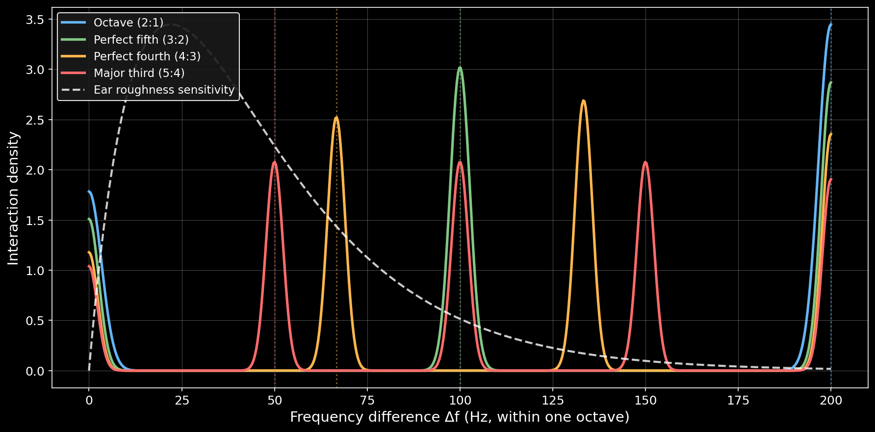
C. Partial–partial frequency differences (interaction density)
Panel C overlays four distributions that explain why the dissonance curve in Panel B has its shape.
For each interval, all frequency differences (Δf) between pairs of harmonic partials are computed. These Δf values are visualized using a kernel density estimate (KDE, with bandwidth parameter 0.035) scaled by the number of interactions, so peak height reflects interaction density per Hz, not probability. The smooth curves result from this kernel density estimation; raw histograms would show discrete bins.
Panel C shows Δf within one octave of the fundamental (0–200 Hz)—this range was chosen because it represents one octave of the reference frequency and encompasses the most perceptually relevant roughness-sensitive region (roughly 20–50 Hz at this pitch, based on an ERB-estimated critical bandwidth of 35–40 Hz at 200 Hz). The dashed black curve overlays the ear’s roughness sensitivity from Panel A as a reference. Vertical dotted lines mark the frequency difference between the two fundamentals (Δf₍fund₎) for each interval. These fundamental differences often fall outside the roughness-sensitive region, which is why consonant intervals aren’t simply those with small fundamental frequency differences—the full distribution of partial interactions matters.
Kernel density estimates showing where harmonic partial interactions concentrate for four musical intervals. The octave (blue) has most interactions at Δf = 0 (aligned partials), avoiding the roughness-sensitive region (~20-50 Hz). The major third (red) has broader overlap with this region, producing more dissonance.
How Panels B and C are related
Dips in Panel B frequently correspond to favorable interaction distributions in Panel C (i.e., distributions with minimal overlap with the roughness-sensitive region), and this relationship is meaningful. However, the panels are not expected to align exactly.
The reason is structural:
- Panel C shows where interactions are concentrated in Δf-space within the displayed range (0–200 Hz).
- Panel B shows the total roughness, which integrates roughness contributions across all frequency differences (including those beyond 200 Hz), weighted by the ear’s roughness sensitivity curve.
In other words, peak position alone does not determine dissonance. What matters is the overall overlap between the complete interaction distribution and the ear’s roughness sensitivity, integrated across all frequencies.
Examples:
- Octave (2 : 1) Because doubling the frequency places every partial of the second note exactly on a partial of the first note, most interactions produce Δf = 0. This creates a very tall KDE peak at Δf ≈ 0 in Panel C. Additionally, mismatched partials between adjacent harmonics of the two tones (e.g., 200 Hz vs 400 Hz, 400 Hz vs 600 Hz) produce a second peak at Δf = f₀ = 200 Hz, visible at the right edge of Panel C. These are the only two peaks visible in the displayed 0–200 Hz range, though higher-frequency differences exist beyond this window. The concentration of interactions at exact alignment (Δf = 0) results in minimal overlap with the roughness-sensitive region (20–50 Hz) and a deep dissonance minimum.
- Perfect fifth (3 : 2) Produces strong interaction clustering with peaks distributed across multiple frequencies, with some overlap with the roughness-sensitive region, yielding moderate consonance.
- Major third (5 : 4) Produces a broader interaction distribution with greater overlap with the roughness-sensitive region (20–50 Hz), yielding higher total dissonance.
Important: Panel B integrates roughness contributions across all frequency differences, while Panel C visualizes only the 0–200 Hz range. Therefore, Panel B is not literally “an integral over Panel C”—it includes contributions from higher-frequency partial interactions not shown in Panel C. However, the displayed range captures the most perceptually significant interactions.
Conclusion
Consonance is not encoded directly in musical ratios, nor in the ear’s roughness curve alone. It emerges from how harmonic spectra distribute their partial–partial frequency differences relative to auditory sensitivity. Panel B summarizes the perceptual outcome; Panel C reveals the interaction structure that produces it.
The fact that these panels are often visually close but not exactly aligned is not a flaw of the visualization—it is the central insight the figure is meant to convey. Only unison collapses to a single Δf value; all other musical intervals generate structured distributions of frequency differences once harmonics are included.
Methods and Limitations
Model specifications:
- Reference frequency: f₀ = 200 Hz (approximately G3)
- Number of partials: 30 harmonics
- Roughness model: Simplified Plomp–Levelt model with constant critical bandwidth (cbw = 100 Hz)
- KDE bandwidth: 0.035 (for Panel C visualization)
Key simplifications:
- Constant critical bandwidth: The model uses a fixed cbw of 100 Hz for all frequencies. In reality, critical bandwidth scales with center frequency according to the ERB (Equivalent Rectangular Bandwidth) formula—approximately 35–40 Hz at 200 Hz, 130 Hz at 1000 Hz, and 550 Hz at 5000 Hz. This simplification affects the accuracy of roughness calculations, particularly for higher partials, but provides a clear demonstration of the underlying principles.
- Equal amplitude partials: All partials are treated as having equal amplitude. Real musical instrument spectra exhibit amplitude rolloff with increasing partial number, which would weight lower partials more heavily in the dissonance calculation.
- Harmonic spectra only: The model assumes perfectly harmonic spectra. Real instruments, especially percussive ones, often have inharmonic partials that would alter the interaction patterns.
- No temporal effects: The model is based on steady-state spectra and does not account for temporal envelope, attack transients, or beating patterns that influence real-world consonance perception.
- Cultural factors: While the psychoacoustic roughness model is universal, musical consonance preferences are partially culturally learned. This model captures the sensory component but not learned associations.
References
This post is mostly a personal exercise in visualizing these concepts. If you want to actually understand musical dissonance, you should check out these excellent resources instead:
-
The Physics Of Dissonance by Henry Reich (minutephysics) Clear, intuitive explanation of the physics behind musical intervals
-
Dissonance: A Journey Through Musical Possibility Space by Aatish Bhatia Interactive tool to explore dissonance by playing with actual waveforms
-
Research Note: Musical Consonance from Frequency Interactions — Adversarial audit of the claims in this post, with primary sources and falsification criteria.
Both are far more accessible and insightful than this technical writeup.
Authorship
I didn’t write any of this content. The text, visualizations, and interactive plots are the result of iterative collaboration and “LLM dueling” between Claude (Anthropic) and ChatGPT (OpenAI). The interactive plots were implemented by Claude Code.
🤖 Created with Claude Code